Traffic Policing And Its Relationship With Income

Introduction

Policing is a rather mixed affair hinging on a number of different factors with some encounters being relatively short and simple while others are more tense and hostile. There are many different reasons for why police make the decisions that they make, either rightfully or wrongfully, many of which aren’t directly observable or easily determined within police data. Some of these factors may include suspicion of drivers doing illegal activity, misdemeanors, or having unconscious bias against individuals that appear to fit their mental description of what a criminal may look like. While racial prejudice is one of the more striking factors to point at when considering how or why encounters between individuals and police officers go differently, decisions seemly motivated by racial bias may potentially be actually due to social class or perceived social class of the individual rather than their race.

For police traffic stops and searches, the assumption here is that a police officer is much less likely to ticket or search a person they consider to be an upstanding citizen. They would be much more likely to search a lower class person who they wouldn’t regard as highly. Police officers would be less likely to suspect a person of drug or other contraband crimes if they perceive the person to be middle or upper class rather than lower class. Based on an officer’s biases they may end up fishing for contraband much more than they should against these drivers, wasting the time of both the officer and the driver as well as potentially increasing the tension or distrust between the drivers and officers.

Stop Outcomes	Driver Has Contraband	Driver Doesn’t Have Contraband
Officer Searches Driver	Search Was Warrented	Search Was Needless
Officer Doesn’t Search Driver	Driver Gets Away With Contraband	No Search Required

Analysis Based on Service Area Income

The dataset we are using is the San Diego Police Stops Data from the Stanford Open Policing Dataset. This dataset gives us data from 2015 to 2019 for all police traffic stops in San Diego county. The county is split geographically into a number of smaller service areas where officers may be stationed to. For this analysis we will be focusing on the search rate of drivers in order to determine if police are biased in their searches based off the driver’s percieved income level.

The first methods we used to to judge a driver’s percived income is using the average income of the service area the police stopped them in. This might not be entirely accurate for say drivers who aren’t from a service area they get stopped in, but what is important here is the police’s perception of the driver’s income level, not necessarily how much the driver actually makes. It should give us a general idea of how police might behave differently in different service areas as well.

In order to get average income of service areas, we used census data of San Diego County which contained information on average income for each geographical census block. Then we joined the correct census blocks that fit or were a part of a service area and took the average from those census blocks for each service area. This is still a rough estimation given how large service areas can be compared to individual census blocks, but overall should be close to the actual average.

In order to get the average income of each service area here we used income data from the 2010 US census. Then we geospacially joined the service areas and the census tracts and got the average of all census tracts within each service area to get the average income of each service area.

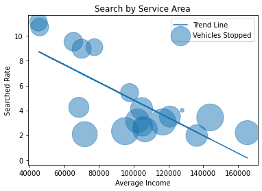
Here we have each Service Area represented as a bubble and we can see that police searched lower income service areas at a higher rate and that the higher a service area’s income the less likely that drivers will be searched. One potential reason is that police treat lower income service areas differently and believe that they have a higher chance of having contraband and thus search drivers there more often. Or maybe the police don’t expect higher income areas to have drivers with contraband.

There may be two outliers below the curve at around 70k, but looking at it geospacially it can be more easily explained later.

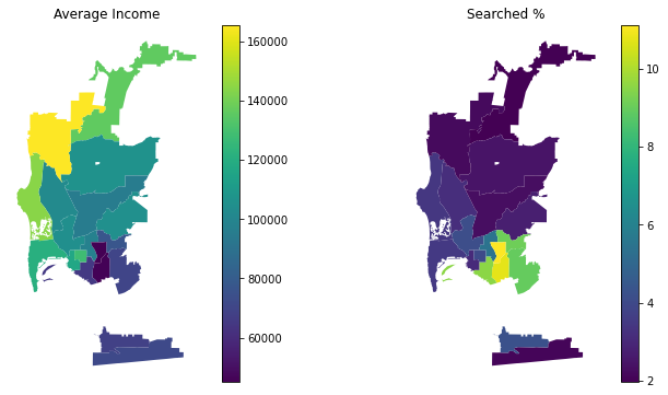
In these geospacial plots, we can see the service areas with the lowest average income near the bottom right of San Diego county. And we see the 5 areas with the highest number of searches also in that area clustered together. This could also point to those 5 clusered Service Areas being more heavily profiled or discriminated against.

The two outliers from before are the ones at the border of San Diego county, where different types of policing may take place for drivers crossing the border.

In these geospacial plots, we can see the service areas with the lowest average income near the bottom right of San Diego county. And we see the 5 areas with the highest number of searches also in that area clustered together. This could also point to those 5 clusered Service Areas being more heavily profiled or discriminated against. The two outliers from before are the ones at the border of San Diego county, where different types of policing may take place for drivers crossing the border.

Veil of Darkness by Service Area Income

Using service area income like in the last section, a technique known as the veil of darkness will be employed.

This technique limits the range of searches to all searches from an hour before twilight to an hour after twilight. After twiight, police cannot as easily racially profile and stop minority drivers since they would not be able to see the color of the driver’s skin. By doing this, we set up a treatment and control group with the treatment being the level of visibility where one group of police officers could racially profile drivers and the other group wouldn’t be as able to. By limiting it to an hour before twilight to an hour after twilight, we are trying to hold other factors constant such as what drivers may be out on the road and differences in policing behavior at different times of day.

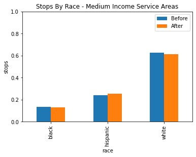
By adding the income of the service areas, we may be able to see a pattern emerge in where this racial profiling is taking place. Different income service areas may have larger populations of African American and Hispanic residents, so racial profiling may be easier for police despite the constraint so we may see less of a difference in those service areas. For this analysis, it made sense to divide the data into three income brackets, and it was settled to be under 80k, 80k to 110k and over 110k. This gets us a low, middle and high grouping where each has a similar amount of service areas.

We are also going to be keeping track of the power of each sample, in order to help note how much confidence we can have in our statistic when we get small sample sizes. This gives us the percent chance that the difference we get is actually accurate or if it could just be due to randomness inherent to smaller sample sizes.

Low Income	Medium Income	High Income

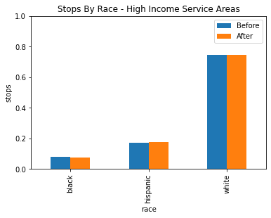After grouping the service areas into three categories based on income for low, medium and high income, there seems to be no statistically siginificant evidence of racial profiling shown through the veil of darkness technique.

Note that veil of darkness only finds explicit racial profiling of specific drivers, so for example there may still be a possibility that racial profiling based on the service areas or other proxies where police may expect the general residence to be heavily minority.

Car Price as a Proxy for Driver Wealth

In order to further our analysis on police stop data, we wanted to explore how police perceive a driver’s wealth, and how that could influence their decisions to stop, search or arrest different drivers. From the Stanford Open Police Project, we found a dataset that includes stop data from San Antonio, Texas, with the make, model and year of the car stopped. I wanted to join this onto a dataset to get the price of the car that was stopped. We found a Kelly Blue Book (KBB) dataset that we could join onto to get car prices. However, several potential problems soon arose: the Texas data abbreviated the make and model of the car. For example, a 2015 Toyota Tundra would be 2015 TOY TUND, whereas KBB uses full names. After some consideration, I elected to go with the KBB data, as it was more complete and included more makes and models of cars.

The Texas data includes over 20,000 unique year, make and model cars, and the KBB data provides price data for 17,651 unique year make and model cars. I first tried to use difflib to find closest matches directly between these two datasets, but the code was too inefficient and would take many hours to run. Difflib.get_close_matches() returns a “close enough” match based on the number of similarities it can find between a string and a list of comparison strings.To work around the large datasets and runtime of get_close_matches, I first made a dictionary that matches the car make as listed in the texas dataset with the car makes in the KBB dataset by hand. The resulting dictionary had 44 matches. I then made an empty dictionary to hold the price of each make and model. Then, for each car in the Kelly Blue Book data, I found the closest match in the texas data to the full car name, (year, make, model), then set that closest match to be a key in the empty dictionary. I then set the value for that key to be the price from the KBB data. I converted that dictionary into a dataset, cleaned it and gave it column names, then merged it onto the texas dataset to get a dataset that has 65217 rows. Overall, the quality of the join is decent, but leaves much to be desired. After cleaning the Texas dataset, it had 873,113 rows with car data in them, but the join reduced that to just 65,217 rows, a reduction of 92%.

Even though there is still plenty of data to be analyzed, it shows that this join method is far from optimal, and is something that can be improved upon in the future. A working hypothesis on why so much data could not be matched is due to a mismatch between KBB and Texas datasets, with KBB not having some cars mentioned in the Texas Dataset. It could also be due to the messy nature of the Texas Dataset, with some cars having wildly incorrect ages, making it impossible to find a similar match with KBB data. After obtaining a joined dataset that includes the police traffic stops and the price of the car stopped, I binned the prices of the cars into three categories to see how search and arrest rates would differ between them. Cheap cars are less than 10,000 dollars, medium cars are between 10,000 dollars and 35,000 dollars, and expensive cars are anything more expensive than 35,000 dollars. What I found was that cheap cars had much higher arrest and search rates when compared to expensive and medium priced cars. Cheap cars had an arrest rate of 0.237%, and a search rate of 0.77%, when compared to expensive and medium priced cars, which had arrest rates between 0.11% and 0.13%, and search rates between 0.26 and 0.276%, a significant decrease in rates that is indicative of some bias in policing towards cheaper cars.

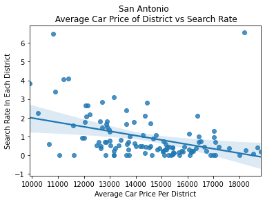
To dive deeper into the correlation between driver wealth and police action, I looked into any potential correlations between the average car price in each district and the search and arrest rates in each district.

Car Price vs Search Rate	Car Price vs Arrest Rate

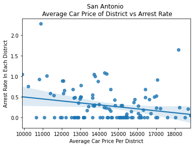After plotting these variables, I found strong negative correlations between them, showing that as car price increases, the search rate decreases.

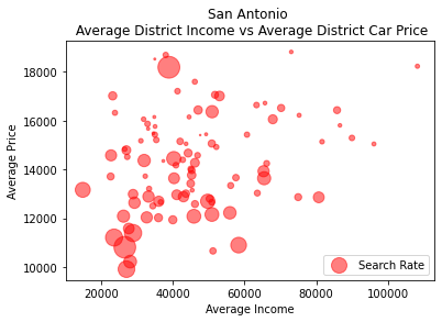
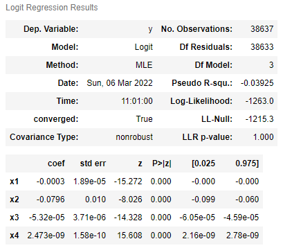
We can see here in the graph above that as the average price of a car and the average income of a district increases, we see the search rate begin to shrink. To further investigate this correlation, I ran a logistic regression on these variables: car price, car age, income of the area the car was stopped, and the product of the car price and income of the area to predict the search and arrest rates.

Logsitic Regression on Searches	Logsitic Regression on Arrests

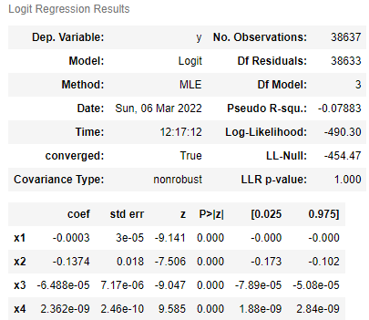We can see that in both models, each coefficient is close to zero. We can calculate the odds ratio that associates each variable with whether that driver will be searched or arrested or not. For each coefficient we see that:

Variable	Search Rate Odds	Arrest Rate Odds
Price	0.9997	0.9997
Age	0.9235	0.8716
Income	0.999	1.000
Price * Income	1	1

This means that for each increase in price of car, or age of car, or income of the area, will multiply the odds of being searched or arrested by the corresponding value in the table above. For example, each dollar increase will multiply the odds of being searched by 0.9997, which is a slightly downwards trend. We can see that the age of the car has the largest downwards trends, with multipliers of 0.9235 and 0.8716 for search odds and arrest odds respectively.

In order to compare how drivers were being treated based on their cars more directly, we looked at the cumulative distribution function, or CDF, of the prices of cars that were searched and the prices of all cars that were stopped. The cumulative distribution function by car price will let us see what proportion of cars in the data are less than or equal to any given price in the data. So for example if 50 percent of cars were under 15k in price, then that would give us a y-value of .5 and an x value of 15k. So not only will this give us the general price distribution of all cars in the populations, but it also lets us see how well the searched and stopped distributions match.

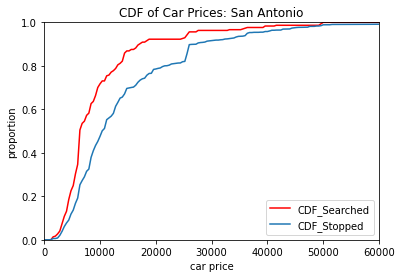
With a p-value extremely close to 0, there is statistically significant evidence of that lower priced cars searched at a higher proportion than they are stopped.

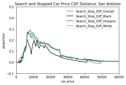
Looking at the Search and Stopped CDF by difference value, we see that both hispanic and white drivers match up closely with the overall CDF difference, but Black drivers have a sudden dip around 10000 and overall have less of a search and stop CDF difference. This is most likely due to us not having enough data as with only 42 Black drivers total that were searched, we have a few potential hypotheses on how this could happen in general.

One possibility could be that low income Black drivers are less likely to give consent to a police officer to search their car, and so police cannot legally search them without some other reason to justify their search. This could have some merit in some areas where Black drivers and police officers have a more tense relationship or have a history of bias against Black drivers. Or even news report of events of police brutality and discriminatory practice of police against minorities could lead to Black drivers not wanting to allow police to search their car for a reasonable fear of being discriminated against.

Another possibility, although one that we’d suspect to be highly unlikely in this case, is that a police officer’s decision to search Black drivers specifically is not as affected by the price of the car. It could be possible then that searches car CDF would match the stop CDF if and only if the police officer do not care or account the price of the car in their decision to search specifically because the driver is Black.

The general bias towards searching cars that are of a lower price is still mostly prevalent across the groups of drivers.

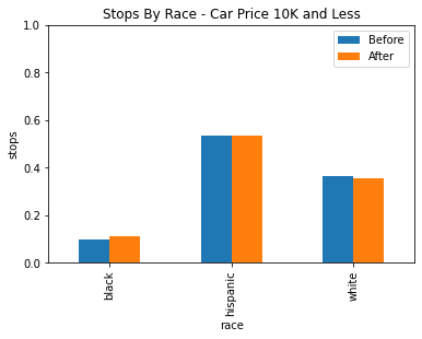
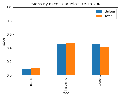
Similar to Veil of Darkness using Service Areas, we can use veil of darkness while grouping cars of different price ranges in order to control for the effect of car price on racial profiling.

Unfortunately, the downside to using the veil of darkness here is that there isn’t quite enough data in the dataset to come to any strong conclusions. The data was divided into three groups, under 10k, 10k to 20k, and above 20k.

Under 10k	10k to 20k	Above 20k

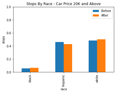Based on the data we have still, there isn’t any statistically significant evidence for racial profiling after factoring in car price. While there does seem to be a statistically significant decrease in the stop rate of white drivers between 10k and 20k, it may be more likely that is due to some other confounding factor or factors.

We also have very low power in our statistics for black drivers because of the low amount of black drivers here, so we cannot draw any notable conclusions for or against racial profiling in any of these groups.

Feedback Loop Simulation

When we are preparing the Stanford Open Policing Data, we try to rule out columns that we think are not features that a police officer can come up with at the time of the stop if they wish to use our model. We decided to stick with 9 features, all of which are reasonable in that a police officer is able to pull up all the information necessary to input into the model. For example, we have the service area, a police officer should know which area they are currently assigned to, we have race/sex/age that can be pulled up from the license plate (only correct if the person driving is who the car is registered to), and day of the week.

While cleaning and preparing our data, we are also trying to make our label/prediction much better. For example if our initial data had been a search but there was no contraband found then in our newly created label we would have a 0 meaning there should not have been a search in the first place.

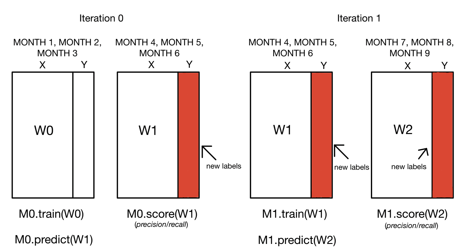
So how our model works is that it takes in the first n months (lets use 3 in this example) and trains the model on those first 3 months of the dataset. Then we take the next 3 months (Months 4-6) and predict on that. When we have those predictions we then replace the actual labels of Months 4-6 with the predicted labels and we refit the model with Months 4-6 and the predicted labels and then we take the 3 months after (Months 7-9) and do the same until we reach the last months of the dataset. We evaluate our model using recall and precision, as well as accuracy. The current Classifier we are using is LDA, but we will keep trying out different models to see which works best. When we get predictions, we do some modification to get better Y’s. If the model predicted 1, and it is actually 0, we change the label to a 0. If the model predicted 1 and it is actually 1, we keep the label of 1. If the model predicts 0 and it’s actually 0, we keep the label of 0. Finally, if the model predicts 0 and it is actually 1, then we flip the label to 0.

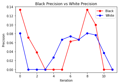
We see that our model is predicting to search more white people than black people regardless of having race as a feature or not while training the model. We believe that this is happening because only ~19% of the data we have is black drivers. It is also predicting searches mostly in service area 120. This service area consists of La Jolla, Torrey Pines, Pacific Beach, and Mission Beach. Although this is not a feedback loop that deals with race, the fact that searches are mainly being predicted in this area could be indirectly correlated to the race of the drivers in this area.

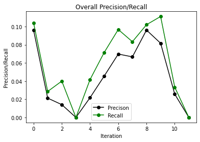
Overall Precision and Recall	Precision	Recall

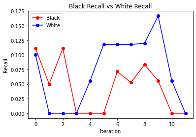The 3 graphs we have here are for when we give the model race as one of the features as well as only have it take in 3 months at a time. Between recall and precision, we see they kind of have a similar pattern, they are 0 for 3 iterations towards the beginning and then they both end up at 0 for both black and white drivers. The precision/recall overall is low toward the early iterations and then it gradually goes up in the later iterations.

If this model were to be deployed, we would expect police officers to use it if they had someone stopped and were trying to figure out if they should search them or not. The inputs to the model would all be available to the officer performing the stop, therefore the model should be able to give a good prediction of whether or not the officer should search or not. We came to the conclusion that there was no positive or negative feedback loop happening in our model. The recall and precision graphs do not give us enough evidence in order to support if there is a feedback loop or not.

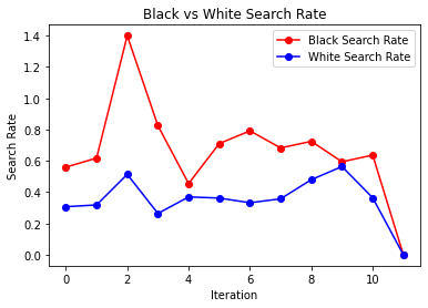
We also took a look at search rates after each iteration, we saw that black search rate was for the most part always higher than white search rate, but as we go through the iterations we see that it stays constant and does not increase (at times there are some spikes). If a negative feedback loop did exist, we would see the search rate increase.

Conclusions

There is evidence of search rates being correlated with a driver’s percieved income based on the service area or the price of their car. We also see that these drivers may be getting unfairly searched when you look at the arrest rates after searches or that police may be fishing for contraband much more than they should be. There is also evidence that cheaper cars get searched more often than they are stopped and that this trend is seen across the three racial demographics that we looked at.

In conclusion, we have found that police search and arrest rates have a significant correlation with the perception of a driver’s wealth. As the average income of an area and the average car price of an area increases, the search and arrest rates of those areas decrease accordingly. After running logistic regression on a car’s price, age, and income of the area it was stopped in, we find that each variable has small yet significant impacts on the probability of a driver being stopped.

In terms of racial profiling, even after controlling for service area income and car price seperately, we were unable to find any notable evidence of racial profiling of stops. While this is interesting and we see income potentially playing a larger effect than racial bias in this data, these results are only limited to San Diego and San Antonio and we might expect to see different results if we were to look at other cities with large minority populations or those with histories of racial profiling by police.

Discussion

Overall we have seen some evidence of correlation between a driver’s income and the likelihood of them being searched. However we are not able to draw many strong conclusions due to an overall lack of data. Car price does seem like a reasonable proxy for driver wealth and using car make and model to find them has been able to get us car prices with good accuracy. However there are actually very few data sets that give car make and model consistently that we could find, with the datasets that do provide it only having it for roughly 20 percent of the data on average. If more policing data had this statistic though we think that there is more that can be uncovered.

Something else to consider is having the service areas be more publicly available in the form of shape files. One issue we ended up running into using the San Antonio data were that they had their data groupped into six larger areas or hundreds smaller areas, neither one was really as useful as they could potentially be because the number of stops and searches in each individual area were too small to get statistics from or were grouped so much that it made it difficult to determine a meaningful trend.

While we did not find conclusive evidence of racial profiling here, looking into other cities may yield different results using these methods. And with how our project was set up we have at least built a general tool that can be applied to other policing datasets.

Links

Here are the links to different resources we used

http://doi.org/10.18128/D050.V16.0: Geospacial Census Data

https://openpolicing.stanford.edu/: Stanford Open Policing Project

https://data.sandiego.gov/datasets/police-vehicle-stops/: San Diego Policing Dataset

https://raw.githubusercontent.com/Tai-Pach/kbb/gh-pages/KBB_used_final_3.csv: Car Data from Kelly Blue Book